If you are reading this blog, then I’d assume you have some basic idea about how neural networks work. If not then I’d recommend you go through this excellent video by Brandon Rohrer. This would make the foundation for what I’m about to discuss.
The code that you see here can be found on my GitHub. I recommend you download the iPython Notebook and play with the code yourself.
Sigmoid
If you are all set, then I’ll start by introducing the sigmoid function. Sigmoid is a type of activation function for artificial neurons in an artificial neural network. It looks like this:
Sigmoid has an output boundary of (0, 1), and α is the offset parameter to set the value at which the sigmoid evaluates to 0. Let’s plot the sigmoid function and then we’ll discuss its usage.
To plot the sigmoid function we need some example data:
import numpy as np
import matplotlib.pyplot as plt

X = np.arange(-10, 10, .2)
Y = np.linspace(0, len(X), len(X))
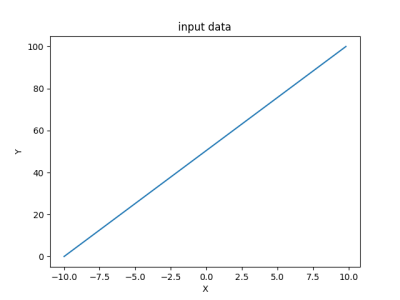
The above code gives us values for X ranging from -10 to +10, with an interval of 0.2. A total of 100 values. And for Y, we have 100 values ranging from 0 to 100.
We can plot this data:
plt.plot(X, Y)
plt.xlabel('X')
plt.ylabel('Y')
plt.title('input data')
plt.show()
The plot looks like this:
Let us now define the sigmoid function and plot sigmoid(X).
def sigmoid(arr, offset):
    a = []
    for x in arr:
        a.append(1 / (1+np.exp(-x+offset)))
    return a

S = sigmoid(X, 0)

plt.plot(X, S)
plt.xlabel('X')
plt.ylabel('Y')
plt.title('sigmoid')
plt.show()
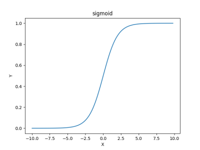
Here’s the plot:
Again, Sigmoid?
- An activation function that turns linear inputs to non-linear outputs. (The non-linearity of Y is observed in the above plot.)
- Bounds the output between 0 and 1 so that it can be interpreted as a probability.
- Real-valued and differentiable. (We need this differentiability in order to perform gradient descent, which is a topic for another day.)
Sigmoids work like a charm for gradient descent (we perform gradient descent to reinitialize the weights for our artificial neurons so that our prediction gets better) as long as X is kept within a limit. Observe the plot. For large values of X, Y is constant. Thus, dy/dx (the gradient) equates to 0. This is termed as the “vanishing gradient” problem.
This is a problem because when the gradient is 0, multiplying it with the loss (actual output - predicted output) also gives us 0. And the networks stops learning as, essentially, learning in case of gradient descent is adjusting the weights for the neurons by adding the previous weight with the loss multiplied by the gradient.
DON’T PANIC. There’s a way around.
See what happens when we sum many of these sigmoid outputs, all computed with a different offset (α).
nb_sum = 10 # number of logistics to sum
offsets = np.linspace(0, np.max(X), 100)

S_sum = np.zeros(np.shape(X))

for offset in offsets:
    S_sum += sigmoid(X, offset)

S_sum = S_sum / nb_sum

plt.plot(X, S_sum)
plt.xlabel('X')
plt.ylabel('Y')
plt.title('Sum of sigmoids')
plt.show()
You’ll be surprised by the output:
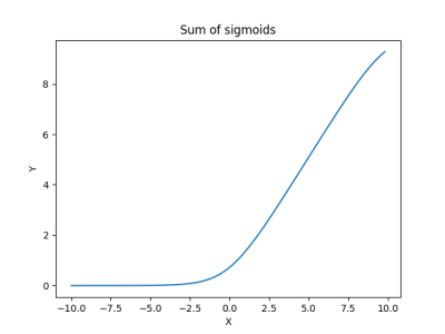
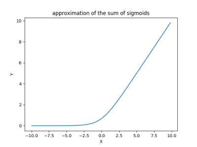
The gradient does not vanish, anymore. But computing these many sigmoids is not really a good idea. It turns out that we have an even better way to do this. Here is an approximation of the sum of sigmoids that we have just computed,
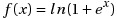
Let’s define the function and plot it.
def sigmoid_approx(x):
    return np.log(1 + np.exp(x))

S_approx = sigmoid_approx(X)

plt.plot(X, S_approx)
plt.xlabel('X')
plt.ylabel('Y')
plt.title('approximation of the sum of sigmoids')
plt.show()
(The output plot might look familiar.)
But do we really need the log and the exp, or could we just take max(0, x)? .. And that works fine. Behold the Rectified Linear Unit.
ReLU
“Roses Are Red. Violets are Blue. Sigmoid is Good. But I do ReLU.” - Some dude on arXiv
In context of artificial neural networks, a rectifier is defined as,
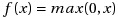
This is also known as the ramp function. Or, more appropriately, the activation function for the lazy engineers (ud-730 reference).
Let’s plot.
def relu(x):
    return np.maximum(0, x)

relu1 = relu(X)

plt.plot(X, relu1)
plt.xlabel('X')
plt.ylabel('Y')
plt.title('ReLU')
plt.show()
The output,
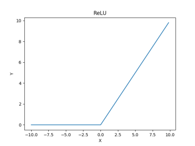
No one’s perfect. ReLU has its problems. The problem with ReLU is that the mean output is not 0. A positive mean introduces a bias for the next layer which can slow down the learning. If the mean value of activation is 0 we get a faster learning.
No one’s perfect, but Jean-Luc Picard.
ELU
With Exponential Linear Units (ELU), we can have a mean activation that is close to 0 and it is an exponential function. ELU does not saturate for large values of x. It is expressed as,
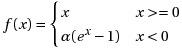
Here α is a parameter. See: https://arxiv.org/abs/1511.07289
In plain English, it acts like a ReLU unit if x is positive, but for negative values it is a function bounded by a fixed value -1, for α=1. This behavior helps to push the mean activation of neurons closer to zero which is beneficial for learning and it helps to learn representations that are more robust to noise.
def elu(arr, alpha):
a = []
for x in arr:
if x >= 0:
a.append(x)
else:
a.append(alpha * (np.exp(x)-1))
return a
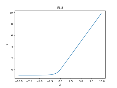
elu1 = elu(X, 1.0)
plt.plot(X, elu1)
plt.xlabel('X')
plt.ylabel('Y')
plt.title('ELU')
plt.show()
Here’s how it looks like,
And here’s 10 hours of non-stop Cantina Band: